Longitudinal Biomarker Tracking and Intraindividual Variability

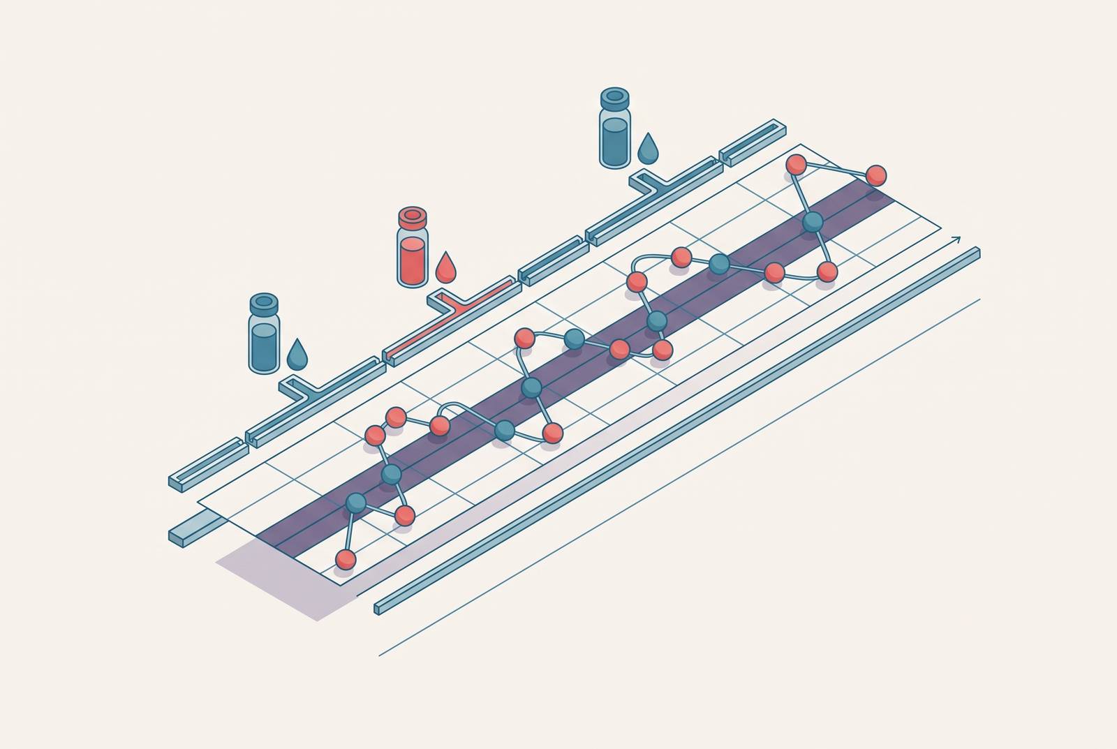
Longitudinal biomarker tracking has spent decades asking one question: does the number go up, down, or stay flat over time? That focus on the mean trajectory misses something else sitting in the same data, the scatter within a single person across repeated draws. That scatter, known in the literature as intraindividual variability (IIV), is the spread across a set of readings, distinct from a single reading or the group average. It's the shape of the noise around a person's own trend line, and the mean trajectory should stop being treated as the whole story, because the shape of that noise carries diagnostic weight the trend line can't.

The field distinguishes two forms. IIV-D, for dispersion, captures inconsistency across cognitive tasks measured within a single session, a snapshot of how uneven someone's performance is at one time point. TB-WIV, or trajectory-based within-individual variability, is newer and harder to pin down: it measures the curvature, the roughness, of a latent biomarker trajectory as it unfolds across visits over months or years. Both push against an assumption that has run biomarker analysis for decades, that the scatter left over once you've drawn the trend line is just noise, safe to average away. That assumption is wrong often enough that it's worth abandoning as a default, not just questioning at the margins.

Why the mean trajectory alone can miss early pathological signals

Two people can post nearly identical slopes on a biomarker chart, same rise, same plateau, and still be walking very different clinical paths. Only one of them may carry a fluctuation pattern that flags disease already at work underneath a trend line that looks calm.

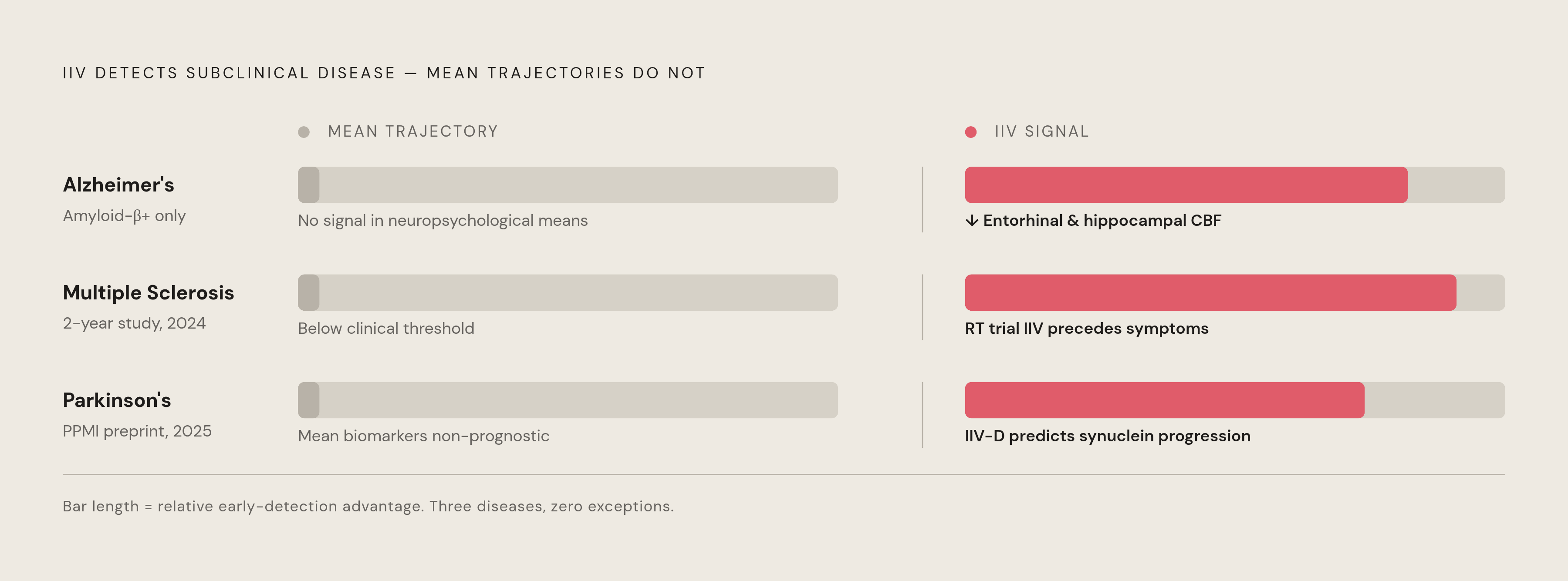
Alzheimer's disease is the clearest case. IIV across neuropsychological test batteries within a single session has emerged as a promising marker for predicting cognitive decline and progression to AD. A 12-month study drawing on the ADNI cohort, 53 non-demented participants who underwent lumbar puncture at baseline along with neuropsychological testing and MRI at baseline and again at 12 months, found that increases in IIV tracked with reductions in entorhinal and hippocampal cerebral blood flow. But that link only showed up in the 21 participants who were amyloid-beta positive, based on their CSF p-tau/Aβ ratio. Among the 32 who tested negative on that biomarker, there was no association at all. The split matters: it means IIV isn't a generic marker of aging or noise, it's tracking something biologically specific.

What makes this finding worth taking seriously is that it held up after controlling for change in mean neuropsychological performance. IIV was carrying information the trend line simply didn't have. And the association was narrow in a telling way: IIV tracked with reduced cerebral blood flow but showed no relationship to cortical thickness or brain volume, pointing toward a mechanism that structural imaging alone would not have detected.

The pattern repeats outside Alzheimer's. A two-year observational study published in 2024 found that IIV in continuous reaction-time trials could catch early cognitive changes in multiple sclerosis before those changes became clinically apparent. An October 2025 preprint from Combs, Kurth, Nair, York, Weintraub and colleagues, drawing on the Parkinson's Progression Markers Initiative, used IIV-D to predict early progression of synuclein disease. Three different diseases, Alzheimer's, MS, Parkinson's, and the same story each time: IIV picks up subclinical or prodromal change well before mean-level scores move enough to register on a chart.

The measurement error problem that complicates every IIV estimate

Measuring this cleanly is hard. Visit-to-visit variability in a biomarker can't be read straight off raw data without running into a basic confound: is the fluctuation biological, or is the assay just imprecise?

If a model specifies a complex mean function to capture the biomarker's trend, whatever within-individual variance is left over tends to be dominated by measurement error rather than biology. Research published in Biostatistics (Oxford Academic) says so directly: how much of the observed within-individual variance reflects real physiological signal, versus assay noise, remains genuinely unsettled in many study designs.

Simple summary statistics like the per-person standard deviation or coefficient of variation are easy to compute, and that ease is exactly the problem. They can't capture variability that itself shifts over time. Worse, when they get plugged into survival models or event-prediction models as covariates, their association with outcomes suffers from regression dilution, a systematic bias toward zero that understates the real effect. Their precision also depends on how many visits each person contributed, and in most clinical datasets, that number is low.

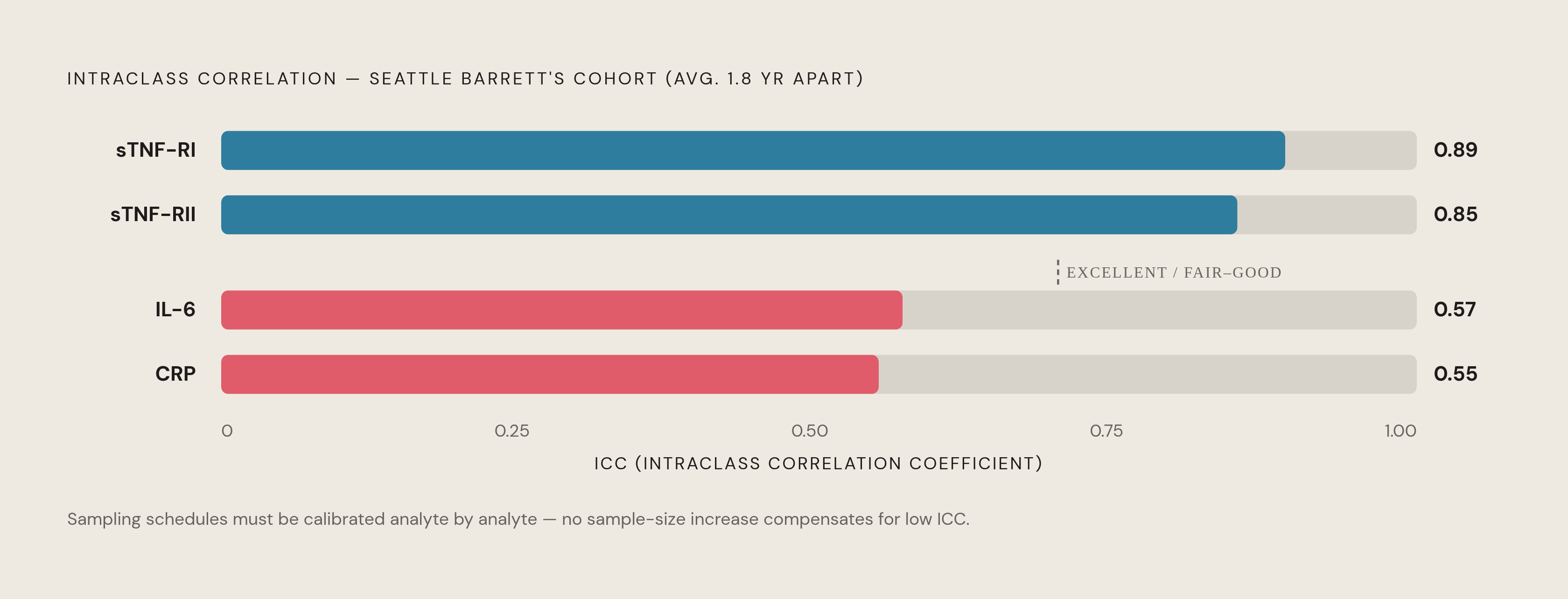
Biomarker choice makes the problem worse, not better, no matter how the sampling is designed. A study using the Seattle Barrett's Esophagus cohort, with samples collected on average 1.8 years apart, found excellent temporal reliability for a class of soluble inflammatory receptors (ICC of 0.89 for sTNF-RI, 0.85 for sTNF-RII) but only fair-to-good reliability for CRP (ICC 0.55) and IL-6 (ICC 0.57). Run the same IIV calculation on a high-ICC analyte and a low-ICC one and the signal-to-noise ratio comes out completely different, a design fact no amount of extra sample size fixes. Post-hoc approaches carry their own risk too: immortal time bias can creep in when variability is summarized as a time-fixed covariate derived from follow-up observations.

Statistical models built to separate true biological variability from noise

A handful of statistical frameworks now try to pull true biological fluctuation apart from measurement noise directly, instead of hoping it sorts itself out in the wash.

The mixed-effects location-scale model (MELSM) is one answer, and it should be the default over ad hoc summary statistics whenever the data supports it. It introduces a random within-individual variance term, so each person gets their own estimated variability level, separate from their own mean trajectory. That error-free variability estimate then feeds into a survival submodel as a predictor, which breaks the chain that causes regression dilution in simpler analyses: variability gets modeled jointly with the trend, not computed afterward as a leftover statistic.

Joint models for longitudinal and time-to-event data have a related blind spot in their standard form: they typically capture only the expected biomarker value and assume residual variability stays constant across people and over time, exactly the assumption IIV research keeps contradicting. Fully joint extensions that model within-subject variability directly do exist, but they're computationally heavy and need dedicated software most clinical biostatistics teams don't have sitting on the shelf. A more workable alternative, proposed in a 2025 arXiv preprint (2605.05923), runs in two steps: derive subject- and time-specific variability measures from the residuals of a mixed-effects model, then feed those measures into a standard joint model alongside the mean trajectory. Less elegant than a fully joint solution, but it still gets you hazard associations without custom software.

Bayesian methods add another layer. Penalized splines (P-splines) and functional principal component analysis have been applied to TB-WIV estimation in a semiparametric framework published in July 2026. Subject-level cubic B-splines, sharing information across individuals for both residual and random-effects variability, handle the data density that intensive longitudinal designs produce, an approach detailed in a 2024 Statistics in Medicine paper out of the University of Michigan. Bayesian mixed-effects models more broadly allow simultaneous inference on intraindividual, interindividual, and population-level variation, three layers that only separate cleanly when the model is built from the start to keep them apart.

A cystic fibrosis mortality study makes the case concrete. Palma and Keogh, working across the MRC Biostatistics Unit at Cambridge and the London School of Hygiene and Tropical Medicine, applied a Bayesian multivariate joint model to a cystic fibrosis registry dataset and found that within-individual variability in multiple markers showed positive associations with mortality risk, findings a model that treats variability as a nuisance would simply never surface.

The clinical tool built on IIV: reference change values and personalized reference intervals

IIV isn't just a research curiosity. It underwrites a working clinical tool: the Reference Change Value, or RCV, a threshold built from analytical precision and a person's own biological variability. A change between two serial measurements has to clear that threshold before a clinician can call it real, rather than noise the assay and the person's own biology would produce anyway.

Serial monitoring often runs on Z-values calculated from analytical precision, intraindividual biological variability, and the RCV together, with clinical events reviewed against that combined framework. Personalized reference intervals, or prRIs, push the idea further. Instead of comparing a patient's result to a population-wide normal range, a prRI anchors the normal range to that patient's own historical baseline. Published biological variation data is the recommended source for calculating these intervals, and RCV can serve as a supplementary check alongside them. Recent literature backs real clinical value in this approach.

The standards underneath all this are still in motion, which matters for anyone tempted to treat RCV thresholds as settled science. A 2024 paper in a clinical laboratory science journal by Jones, Aarsand, Carobene and colleagues (2024; 70: 1076-1084) introduced "regression to the population mean" as a new concept for RCV calculation, a sign that consensus on how to set and interpret these thresholds hasn't arrived yet. And the stakes go past diagnostics. A January 2025 paper in JACC by Gaba, Rosenson, López and colleagues examined intraindividual variability in serial Lp(a) measurements among placebo-treated patients in the OCEAN(a)-DOSE trial, a context where variability in the biomarker itself directly shapes how a drug's effect gets read during development.

What dense, high-frequency data collection reveals that sparse clinic visits cannot

Conventional biomarker sampling, saliva, serum, urine drawn at a clinic visit, is episodic and often invasive, and it catches a single point in time rather than the dynamic variation unfolding over hours or days. Running collection outside a clinical setting is logistically hard, and even when it works, the resolution is too coarse to tell a normal circadian dip from acute physiological strain.

Ecological momentary assessment (EMA) narrows that gap. EMA studies have linked moment-to-moment cognitive fluctuations, captured outside clinic settings, to neurodegeneration biomarkers in ways that sparse sampling would obscure. A monthly or quarterly clinic visit would have averaged that variability out of existence.

Wearable biosensors push the idea further still. Continuous, non-invasive measurement of hormones such as cortisol and melatonin from sweat is now possible, which opens the door to tracking endocrine activity across a full day instead of one blood draw. A wearable sweat-sensing platform described in a paper in Bioengineering & Translational Medicine used a CatBoost Regressor to predict hormone levels from sweat, hitting R² values of 0.984 for cortisol and 0.955 for melatonin. A separate study of 59 participants used Garmin Fenix 6 smartwatches to track physiological and activity data in free-living conditions, demonstrating automated health monitoring outside a clinical setting. And an advanced wearable CRP patch, combining iontophoretic sweat extraction, microfluidic sampling, and a graphene-based sensor array, has been proposed for picomolar-level CRP detection in COPD, heart failure, and infection monitoring.

Chronic kidney disease shows where this approach runs out of road. CKD isn't a single-biomarker disease; it involves multiple metabolic and physiological processes running at once, and wearable translation stalls here precisely because the IIV signal isn't sitting in one analyte, it's spread across several. Population-level differences in age, sex, and stress response pile on another layer of variability that dense data exposes rather than resolves. More data points don't simplify the picture. They make stratification by subgroup more necessary, not less.

How sampling design choices determine whether IIV is recoverable at all

More frequent sampling sounds like it should always help. It doesn't, and treating "more data" as an unqualified good is one of the sturdier myths in this field. A Bayesian mixed-effects analysis of hormonal data from 35 pubertal girls followed over roughly two years, published by Keith, Corley, Glass, Valeggia, and Martin in a human biology journal in 2026, tested nine different sampling schedules: annual, biannual, and quarterly intervals, each with one, two, or three repeated samples per interval.

The result: past a certain point, adding more measurements made individual parameter estimates less precise, not more. Standard errors, credible intervals, and overall residual error moved in ways specific to the biomarker being tracked, and no single sampling schedule won across all of them. Intraindividual, interindividual, and population-level variation have to be modeled as separate layers, and folding them together produces biased estimates no matter how much data goes in.

The Barrett's Esophagus ICC findings apply here too. A sampling interval that suits a high-reliability analyte like sTNF-RI will be wrong for a low-reliability one like CRP or IL-6, which means study design has to be calibrated analyte by analyte, not lifted wholesale from one marker and applied to a whole panel. Before trusting any sampling schedule to capture IIV rather than alias it into something that only looks like noise, researchers need to know the short-term fluctuation range of the specific hormone or marker they're tracking. The goal is to maximize the value of the samples collected. It's to find the minimum number that gives full longitudinal coverage, keeps measurement error in check, and preserves honest uncertainty estimates.

What sound IIV-aware longitudinal analysis requires in practice

Treat IIV as a parameter to estimate, not as noise to absorb into an error term and forget, a starting point that is simple to state and hard to skip. A model has to be built from the outset to capture within-individual variance as its own quantity, not backed into after the fact.

From there, the choice of method matters, and the choice isn't neutral. Two-step residual-based approaches and fully joint MELSM specifications both beat post-hoc summary statistics like per-person standard deviation, because they sidestep the regression dilution that quietly undermines simpler methods. Sampling design has to be calibrated to the specific biomarker's reliability profile, not borrowed wholesale from a different analyte or a different disease, the Barrett's Esophagus ICC numbers alone should settle that argument. And dense, high-frequency data, from EMA, from wearables, from repeated clinic draws, only pays off if the underlying model can actually separate intraindividual, interindividual, and population-level variation instead of blending all three into one number that hides them.

This is a different question being asked of the same data, not a technical footnote bolted onto conventional biomarker tracking. Not just where a person's trend line is headed, but how steady the path getting there really is, and whether that unsteadiness is telling you something the trend line alone never could.